Easy (or at least straightforward) Terrain Relief Models
I promised to write up my process for making high-resolution terrain relief model carvings. This is how I currently do it. The process is easy enough that I can prepare a new area in just a few minutes, and for a 150-170mm square carving with a 1/4" ball nose roughing pass and a tapered mill finishing pass at a stepover of 0.25mm or so, the machine time is somewhere in the 2-3 hour range. So, on to the instructions.
Preparing Your Digital Workspace
I spent some time dialing in a workflow for creating my to-scale high-resolution terrain relief models. You may prefer to follow a different process, but by documenting mine, I figure you may have a better place from which to launch into your own tweaks and optimizations. So, to start off, what do I use?
- My Relief Model Tools spreadsheet.
Not necessary, but I attempted to make the mathy bit of the process as smooth as possible. - Digital Elevation Model (DEM) data from USGS.
In the USA, we have access to lots of free public domain data, so I have not investigated other sources. - QGIS 2 and the DEMto3D plugin.
A great tool for working with DEM data, and free.There is a port of the DEMto3D plugin to QGIS 3, but it is not completely functional at last check. It suffers from UI issues that make it much more difficult to use, and since QGIS 2.18 works fine, I have yet to spend the time to grok the new code.
- Meshmixer.
Used to correct model aspect ratio and optionally add a border (e.g. for style or for making models from multiple physical tiles). - PixelCNC.
I like it for doing relief models. It’s got some rough edges and such, but it’s inexpensive and very quick to work with.You can also use MeshCAM if you have it. I downloaded it for a trial, but I have not purchased it. I cannot say whether the generated toolpaths would be better than those from PixelCNC, but it is definitely slower at processing the data.
- Carbide Motion.
Any G-code sender will work, but the probing example at the end describes Carbide Motion v4 specifically to illustrate the procedure.
Defining Your Map Area
Obviously, step one of any relief modeling project is defining the area you want to model. If you’re looking at a general area, you can just choose the corners of a rectangle and jot down the coordinates. (This can be done in practically any mapping program or even with paper maps.) On the other hand, if you’re looking to make a “souvenir” relief model of a particular place including various waypoints, you’ll want to find the northernmost, southernmost, easternmost, and westernmost points. From there, you can easily add margins.
If you don’t spend your days in maps and coordinates, there’s a simple method to collect the relevant data from Google Maps. Just go to each point you want to have on your model. In a web browser, right-click and choose “What’s here?” from the menu. The coordinates for that point will be displayed at the bottom of the little info box. If you’re in Google Maps on your phone, long-press on the point to drop a pin, and the coordinates of the pin will be displayed in the search bar. Using any method you find convenient, collect the coordinates of all your points (not bothering with any that you know are in the middle of your desired map). Then just independently take the highest and lowest values for the latitude and for the longitude, and you’ve got your target rectangle.
The way I like to work a project is to start by finding the basic bounding box (northernmost, southernmost, easternmost, and westernmost coordinates). Then I go to the spreadsheet and set “Calculate from:” to “Two corner points”. I enter the two latitudes and two longitudes. That gives me the coordinates of the center point and the height and width of my selection (measured N-S and W-E across the center point, respectively). With the center coordinates in hand, I copy them up to the “Center Point and Size” section and change the “Calculate from:” to “Center point and size”. I can round the height and width up to nice round numbers, adding however much margin I feel looks good (and defining the aspect ratio of the carve). With that, the results box updates to show the four bounds I need to use in the next steps.
Acquiring Your Elevation Data
Go to The National Map’s download system: https://viewer.nationalmap.gov/basic/
On the right side above the map, choose “Coordinates” and enter your four values as the pair of latitudes and longitudes. The map will zoom to a highlight box showing the area you’ve specified.
On the left side, click “Elevation Products (3DEP)” under “Data”. Now use the “Show Availability” links to find the best data available. Start with “1 meter DEM”, and if your area is covered, it will be shaded. If you’re not covered, try “1/9 arc-second DEM” next, as it’s more or less a third the resolution of “1 meter DEM”. If you’re still not covered, try “1/3 arc-second DEM”, which basically covers the entire US with something approximating 10m resolution. Some of the formats only provide IMG output, but if you do have an option for “File Format”, you will want to explicitly choose IMG (Erdas Imagine Image), as it will be the most convenient.
If you’re making a relief map of a large area and using a 1/4" ball nose mill, you probably don’t want to bother with the 1 meter DEM data. You don’t need that much detail, so why would you want to download gigs of data you’re just rounding off. On the other hand, if you’re wanting to make a model of just one smallish mountain and you have 1-meter coverage, rejoice! I personally start with the best data I can, since hard drive space is cheap and download speeds aren’t bad these days.
With your search area highlighted and your preferred DEM variety chosen (as an IMG file), now click the “Find Products” button to do your search. On each result, you can click the “Footprint” link in the “Actions” column to see what that file covers. Choose a data set that covers your selected area, or as many as it takes to cover everything. If your area is split across multiple data sets, you’ll have to do an extra step to combine the data later, but no worries. Download the data, and extract the zip file or files to a folder of your choosing.
Using QGIS To Prep Your DEMs
If you have QGIS 2 and the DEMto3D plugin already installed, open QGIS. If you don’t have it yet, go to https://qgis.org/ to download and install QGIS 2.18. Use the “QGIS Standalone Installer Version 2.18” link, as that installs in just one step (compared to however many it takes to get your desired results via the Network Installer). Then open QGIS and choose “Manage and Install Plugins” from the “Plugins” menu. Search for and install the DEMto3D plugin – you don’t even need to restart QGIS.
If you had to download multiple files to cover your selected area, you’ll need to merge the data before you continue. I like to start by putting all my source IMG files in one folder. Either copy the IMG files (the largest file in each zip), or just dump the full contents of all the zip files into the same folder. (Some files will overwrite others, but the data we care about is in the IMG files, which all have unique names.) With all the IMG files in the same folder, it’s time to merge:
- Go to QGIS and click the “Raster” menu, go down to “Miscellaneous”, and choose “Merge…”.
- Click the select button next to the “Input files” box, change the file type drop-down from “All Files (*) (*.*)” to “Erdas Imagine Images (*.img) (*.IMG)”. Then select all your IMG files.
- Click the select button next to the “Output file” box and choose where to save your merged file, being sure to set “Save as type:” to “Erdas Imagine Images (*.img) (*.IMG)”.
- Leave all the other settings unchecked, except “Load into canvas when finished”, which just saves you from having to load your merged DEM data.
- Click OK to start the merge, then OK when it finishes, and so on all the way back to the main screen. (You can skip the next paragraph – your layer’s already loaded.)
To load your DEM data, click the “Layer” menu, go down to “Add Layer…”, then select “Add Raster Layer…”. Change the type drop down (bottom, far right) to “Erdas Imagine Images (*.img *.IMG)”, then go to where you extracted the zip file (or saved your merged data) to select and open your data file. It’s generally the largest file in the folder, by far. You should now see it displayed as a greyscale height map.
To make things as convenient as possible when generating the model, I like to clip the part of the layer I’m planning to work with.
- From the menu bar, click “Raster”, go down to “Extraction”, and choose “Clipper…”.
- If you have multiple layers loaded, be sure “Input file (raster)” is the layer you’re working with.
- Then click “Select…” by the “Output file” box to choose your output file. Choose a folder, give it a name, and of course, save it as an “Erdas Imagine Images (*.img) (*.IMG)” file.
- Click “Save” to return to the Clipper dialog box.
- Be sure “Clipping mode” is set to “Extent”.
- Take your latitude and longitude bounds (e.g. from the spreadsheet you worked in earlier) and enter them in the four boxes: X is longitude, and Y is latitude.
- Leave “Load into canvas when finished” checked, and your clipped layer will automatically be loaded. (It will also be saved where you specified, so if you want to come back and redo your model, you’ll be able to load it and skip all the earlier steps.)
Creating Your 3D Model
With your data all merged, loaded, and clipped, you’re ready to turn your selected layer into a 3D model saved as an STL file.
- Start DEMto3D and select your layer:
- Click the “Raster” menu, go down to “DEMto3D”, and select “DEM 3D Printing”.
- If you have multiple layers loaded, be sure the “Layer to print” drop-down box shows the one you’re working with.
- Click the “Select layer extent” button (looks like a four-arrowed cross) and choose your clipped layer from the list. The X and Y boxes will be filled in, and you’ll see a red selection box around your layer. Now we fill in the other boxes.
- Fill in the details:
- In the “Length (mm):” box, fill in the final physical size of your model along what a Shapeoko calls the X axis.
- Ignore the “Width (mm):” field – the model height scales with the length field, and DEM data in arc-seconds is distorted and must be stretched (a later step) to make it square in distances.
- Leave the “Exaggeration factor:” field at 1.0 so you get a true model – we’ll do any expansion or compression later.
- In the “Height base” section, choose a value for the bottom of your model and fill in the “Height (m):” field – I always copy the value displayed as “Lowest point:”.
- Now, go back up and enter a value for “Spacing (mm):” in the “Model size” section. This defines the detail in your 3D model STL file. (Think of it as something like stepover, so if you’re planning to use a 1mm stepover, there’s no reason to use a 0.2mm spacing. The STL files can get quite large with small spacings.)
- Copy numbers into the spreadsheet:
- Go back to the spreadsheet and scroll down to the section under “Part Two: Model Scaling”.
- Copy the values for length, base height, lowest, and highest.
- Feel free to ignore the width value, as it is not used.
- Save your STL file:
- Click the “Export to STL” button to save your model. This can take a few minutes if you’ve got a big model and a small spacing. Once your model is saved, we’re done with DEMto3D and QGIS, and we’re off for a quick trip through Meshmixer.
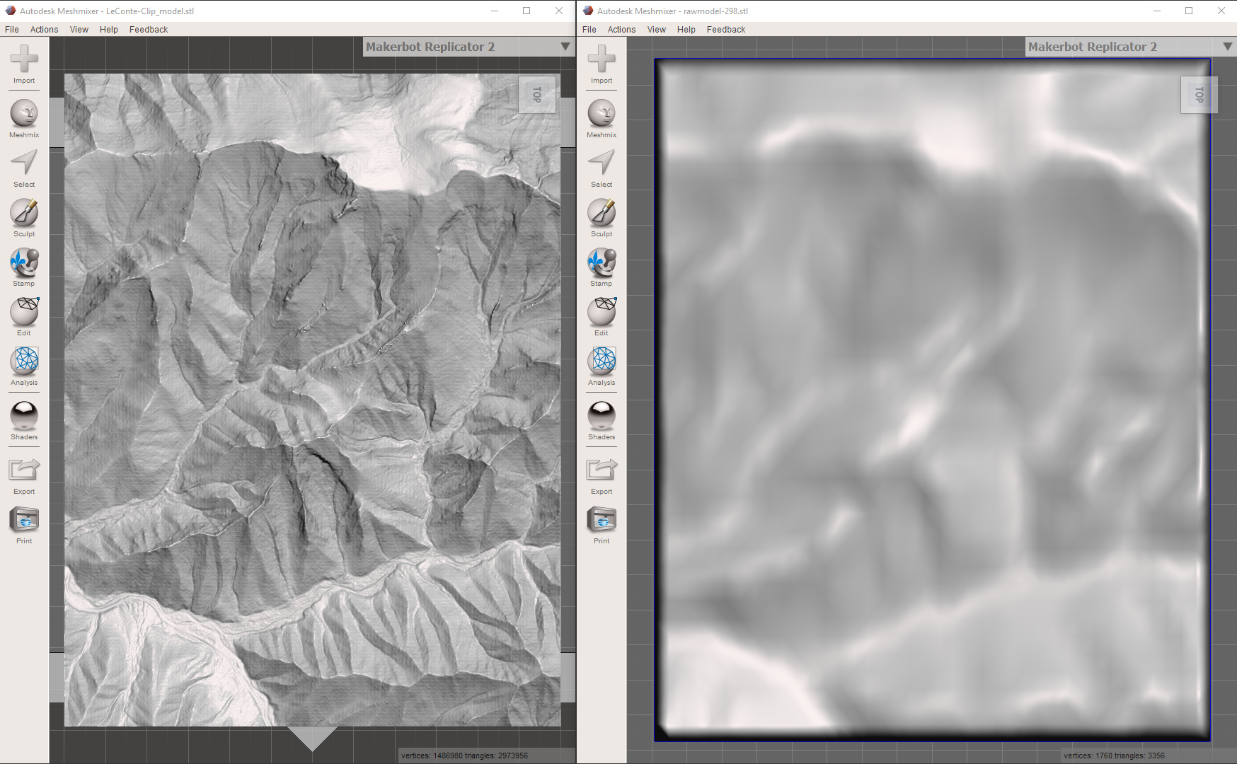
Meshmixer
If you don’t have Meshmixer yet, go to http://meshmixer.com/ to download and install it. Open Meshmixer, and click “Import” to load your newly created STL from wherever you had DEMto3D save it.
First, we need to fix the stretch/squish that came from the file being scaled in lat/lon and not distances. Click “Edit” and choose Transform. Look at the Size X, Size Y, and Size Z values. What you entered as “Length” should be there as the “Size X” value. Now, click on the number next to “Size Z” and replace it with the value for “Model Width” on the bottom of the spreadsheet, being sure “Uniform Scaling” is not checked. You have now successfully scaled the model.
My process of carving the model carves it into a piece of wood, leaving a nice uncarved border around it. If you want to have the surroundings low instead of high, we can do that with a quick bit of Meshmixing:
- With your model selected, click Edit and choose “Align”. This centers your model.
- Click “Meshmix”, then drag one of the solid primitives to the work area. (I generally use the cube.)
- In the Transform dialog that pops up, fill in the three size values (noting that Y and Z are swapped compared to your CNC axes). You can use the “Model Width” and “Model Height” values on the bottom of the spreadsheet as a reference when you’re adding a “border” like this.
- For the “Size Y” (CNC Z) value, note that DEMto3D always adds 2mm to the bottom of the model, using 2mm as the “Size Y” value will make the top of your border the same CNC Z height as the lowest point.
If you want to make a large relief map out of tiles, you can use something less than 2mm as your border. Cut the tiles out on the border and sand off any remaining lip so the tiles fit together just right.
- With your added piece selected, click Edit and choose “Align”. It is now also centered.
- Hold Shift, click to select both the new piece and your terrain model, then click “Combine”.
- Your combined model with border is now ready for export.
With your model’s aspect ratio corrected and any optional border added, you’re ready to save. Click “Export”, and in the “Save as type:” drop-down menu, choose “STL Binary Format (*.stl)”. Give it a name and click save, and you’re done with Meshmixer.
PixelCNC reads binary STLs but not ASCII STLs (like DEMto3D generates), so even if you’re not adding a border or fixing the aspect ratio, you’ll need to import the STL into Meshmixer and export as a Binary STL. If you try to load an STL into PixelCNC and it chokes on it, it’s probably an ASCII STL, so just import into Meshmixer and export as a Binary STL to make everything happy.
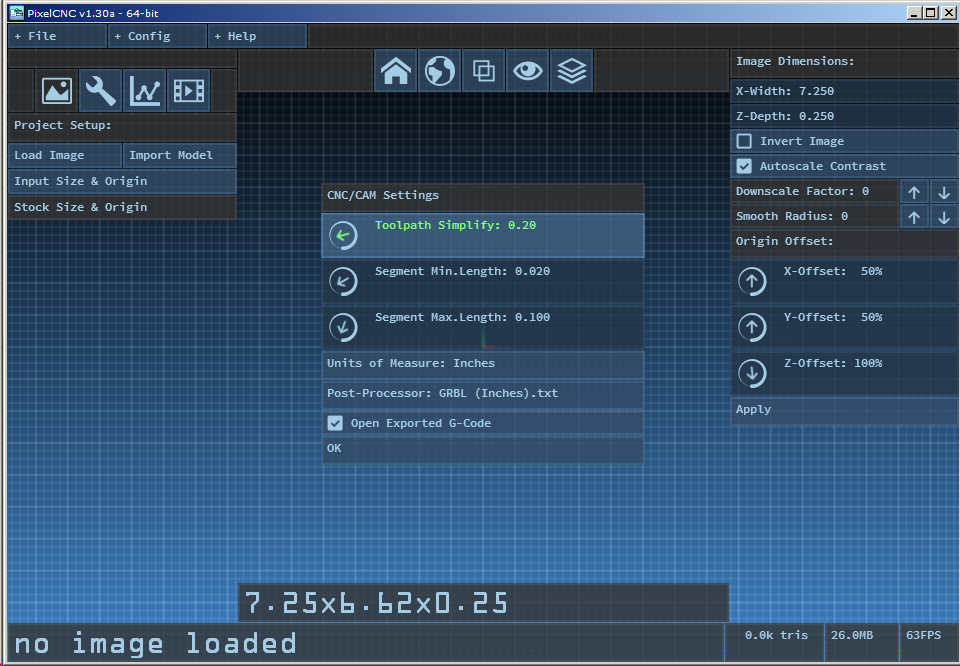
PixelCNC
Open PixelCNC version 1.30 or later, which is available for purchase at https://deftware.itch.io/pixelcnc (or skip this section and use MeshCAM if you have strong feelings that way). If this is a new install, go to “Config”, choose “CNC/CAM Settings”, and select your “Units of Measure” and “Post-Processor”. (“Millimeters” and “GRBL (Metric).txt” for me.)
Load and Scale the Model
- Click “Import Model”, then choose the binary STL you just saved.
- Click “Input Size & Origin”.
- Set the X-Width to your value for “Model Width” from the spreadsheet, or use the final size if you added a border in Meshmixer. (The model will be scaled uniformly in X and Y.)
- Set the Z-Depth to your value for “Model Height” from the spreadsheet. (Adding a border the way it’s described above in the Meshmixer section does not change this value.)
If you want to compress or exaggerate the Z axis, change the “Relief Scale Factor” in the spreadsheet. It will show you the resulting values for “Model Height” and “Total Cut Depth” (which does not include any border you may have added in Meshmixer). Use the scaled value here for Z-Depth.
- I like setting the “Z-Offset” to 100%, which sets Z0 as the top of the carve, as that makes the output independent of stock thickness.
Do Your CAM Magic
- Define your cutting tools. Ball nose mills are type “Cylinder” with a “Corner Radius” set.
- Then define your milling operations. (I like to do a “horizontal” operation to rough it out using a large ball nose mill and leaving a small amount of stock, then follow with a small tapered or ball nose mill to cut in the detail.)
- Check the simulation, et cetera.
- Click “File” and select “Export G-Code”.
Split The G-Code!
PixelCNC (at least as of v1.30) saves the entire job in a single G-code file, but if you’re using more than one tool (of course you are), you’ll want to split things into separate files. In the G-code file, the section for each tool begins with two lines like “( Tool: 1 )” and “T1 M6” and ends with the lines “( Spindle: STOP )” and “M5”. (Using a different post-processor can change things, of course.) Just save one file for each tool change, cutting out the rest of the (Tool) to (Spindle: STOP) blocks – leave everything before the first (Tool) line and everything after the last (Spindle: STOP)/M5 line. Hopefully an update to PixelCNC will let you export G-code split into files per tool, but it’s just big text files.
On Windows, if you’re not using Notepad++, let me just say that it’s one of the first things I install on a new machine. It’s free, GPL, and just plain great for text editing, even before you start installing fancy plugins.
With that, you’re ready to roll. What a relief!
Notes On Probing
As noted above, I prefer to set my Z0 to top of stock, but since a relief model carve generally involves removing the top, that does mean that setting Z0 requires a little two-step to make tool changes easy and straightforward. This is how I handle it. There are two cases. For Case 1, the stock is too tall for the probe block to fit between the stock and the tool. For Case 2, there is room to fit the probe. (These instructions look long, but that’s just because I’m being extra thorough about going step by step through them.)
Case 1:
- Set the probe block on the leveled wasteboard next to the stock.
- Probe for Z. Carbide Motion sets Z0 as the surface of the wasteboard and moves to Z+31mm.
- Jog to the vicinity of what will be the highest point of your relief model (or just use anywhere if you’re confident the stock is flat and level).
- Manually jog down until your tool tip touches the stock (using the paper trick, backlighting, or whatever other method you prefer).
- Write down the currently displayed Z value.
- Rezero your Z right here, and run your first toolpath.
- After changing to a new tool, set the probe block back on your leveled wasteboard, as you did in step 1.
- Probe for Z. Carbide Motion jogs up to Z+31mm.
- Jog your Z axis to the value you wrote down in step 5.
- Rezero your Z right here, and run your next toolpath. Repeat from step 7 as necessary.
Case 2:
- Set the probe block on the leveled wasteboard next to the stock.
- Probe for Z. Carbide Motion sets Z0 as the surface of the wasteboard and moves to Z+31mm.
- On the “Set Zero” page, click “CLEAR ALL OFFSETS”.
- Write down the new value for Z, which will be some negative number.
- Set the probe on what will be the highest point of your relief model (or just use anywhere if you’re confident the stock is flat and level).
- Probe for Z. Carbide Motion sets Z0 as the surface of the stock and moves to Z+31mm.
If your stock is too tall for the automatic jog to Z+31mm after probing for Z on top of your stock, use the Case 1 instructions.
- On the “Set Zero” page, click “CLEAR ALL OFFSETS”.
- Write down the difference in the two Z values (e.g. subtract either from the other, and use the absolute value).
- Set the probe block on the leveled wasteboard next to the stock.
- Probe for Z. Carbide Motion jogs up to Z+31mm.
- Jog your Z axis to the value you wrote down in step 8.
- Rezero your Z right here, and run your next toolpath. Repeat from step 9 as necessary.
Examples and Resources
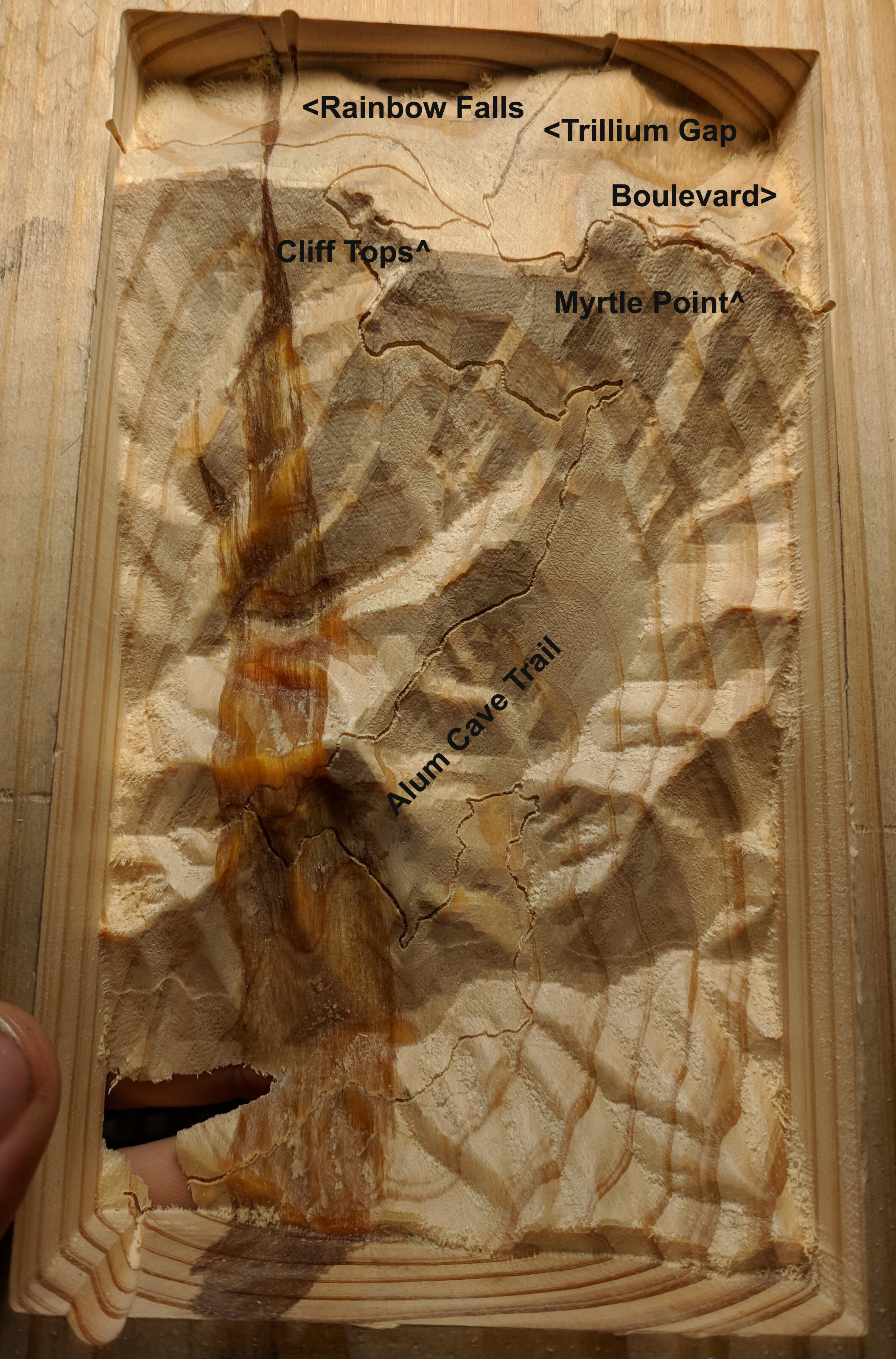
Mount LeConte on a piece of scrap pine 2x6.
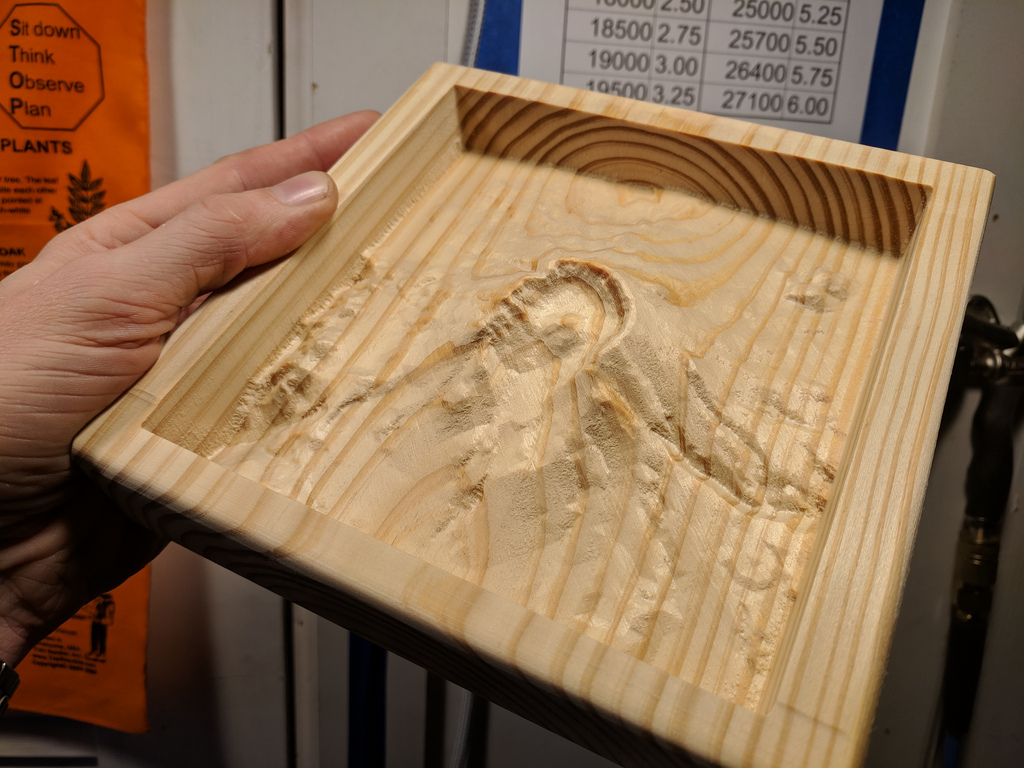
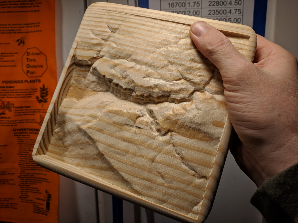
Mount Saint Helens on a piece of scrap pine 2x6.
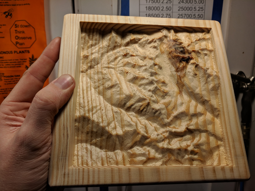
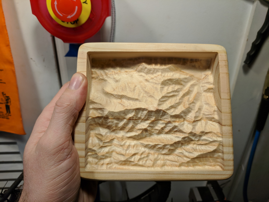
Part of Sequoia/Kings Canyon National Parks (Mineral King is near the bottom left) on a piece of scrap pine 2x6.
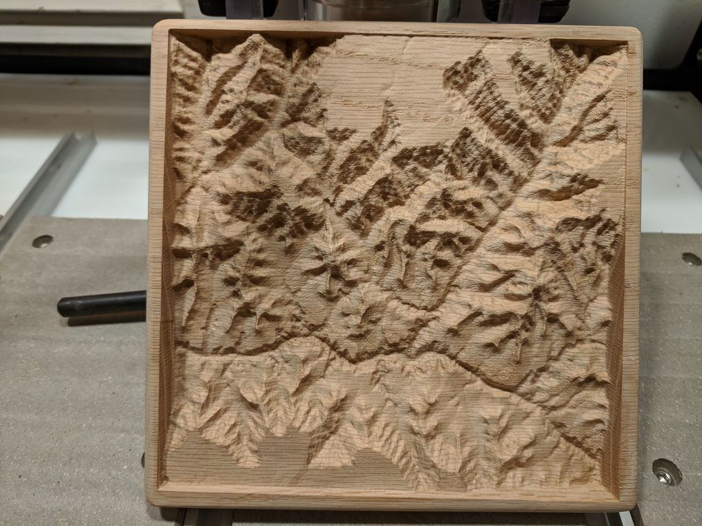
Part of the Grand Canyon on a piece of red oak 1x8. The North Rim Visitor Center is top center. This was by request of a coworker who hiked rim-to-rim (and back, I believe) on the Bright Angel Trail.
ReliefModelTools.zip (7.8 KB) – The same as the Google Sheets spreadsheet, but exported to Excel format to provide an offline reference version.